


lotting the average amplitude of all the traces in a GPR cross-section shows the response character versus travel time (or depth) and provides the user with insights and key understandings of the nature of the data.
In Part 1 of our story about ATA Plots in our July 2018 Subsurface Views, we focused on how to use the Average Time-Amplitude (ATA) plot for:
- Quantifying the level of background noise
- Determining the depth of GPR penetration
- Analyzing GPR signal attenuation with depth
In this article, we continue looking at the power of ATA plots; how they provide insight on the transmit pulse and can help identify coherent system noise and air waves.
Transmitted Pulse
The highest amplitude signal in an ATA plot is normally the direct wave. This signal travels directly from the transmitter to the receiver. In some cases, the direct signal may exceed the maximum value that the receiving electronics can accommodate leading to the peak recorded voltage being less than the true value. This is referred to as signal clipping. When the peak receiver detection level is known, an ATA plot quickly indicates if the transmit pulse (Figure 1) is clipped. The example in Figure 1 shows signals for a receiver with a peak recording range of +/- 50 millivolts. Signals that exceed 50 mV are “clipped” as the plot illustrates.
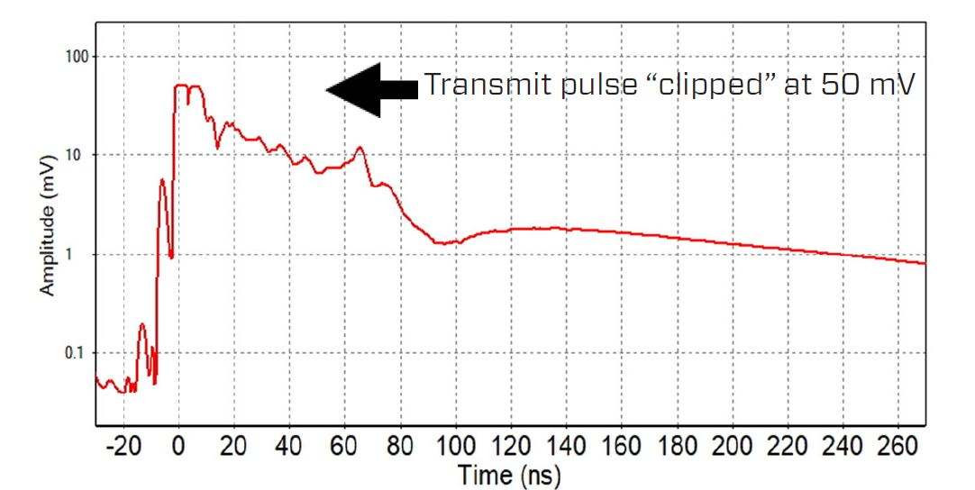
A clipped transmit pulse can affect the use of a background subtraction filter (used to reveal weaker signals masked by the higher amplitude transmit pulse). If data are clipped, target responses in the zone of clipping are not detected. This effect is often referred to as transmitter blanking. If shallow reflectors are not of interest for a given survey, then a clipped transmit pulse is acceptable.
For fully bi-static GPR systems, clipping can be reduced or eliminated by moving the two GPR antennas further apart. Other approaches are to reduce the transmitter power or reduce the receiver gain (and hence receiver sensitivity). All these options are available in the latest pulseEKKO® systems where the user can move each antenna independently, adjust the transmitter voltage or change the receiver gain (in the case of the new Ultra Receiver). GPR systems, such as NOGGIN®, LMX® and CONQUEST® have antennas at a fixed separation and are designed so that signals are not clipped when the system is on the ground.
Coherent Noise
One of the challenging aspects of GPR systems is the presence of time invariant coherent noise. These signals are produced within the GPR system itself and are associated with signals that travel inside the electronics or on the associated cabling and support structure. For extreme cases, these appear as constant bands across a radar section and mask all subsurface responses.
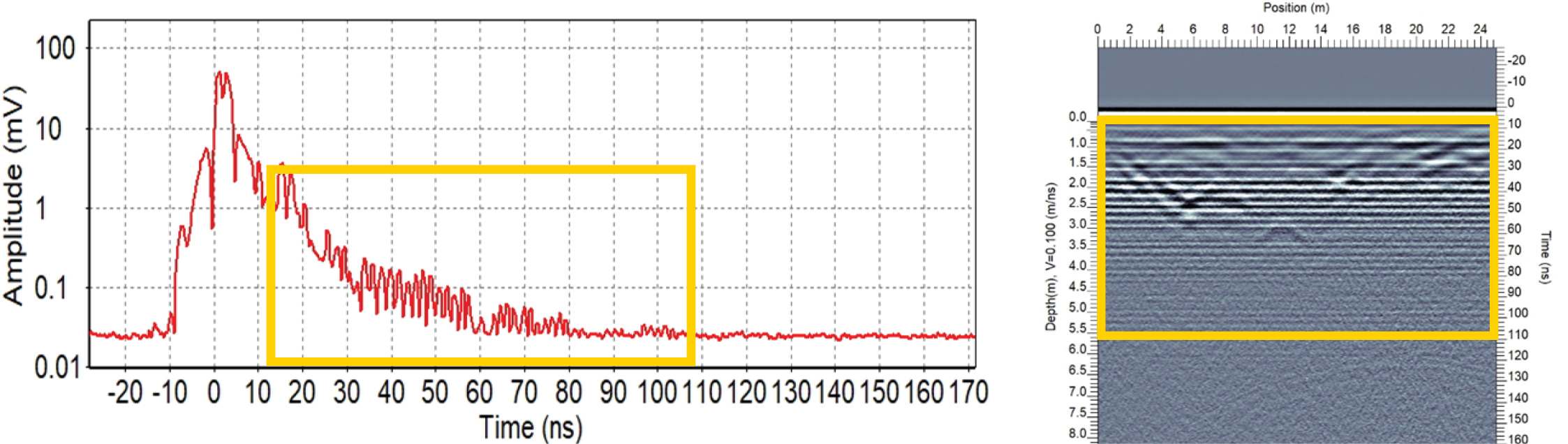
ATA plots are very helpful for assessing the level of time (and spatially) coherent noise. When data are acquired along a transect where there is a substantial amount of change with targets at differing depths and spatial locations, the ATA plot should reveal a smoothly decaying response. The presence of localized peaks on the decaying response curve is indicative of coherent noise.
Figure 2 shows an ATA plot with an example of coherent system noise in the form of periodic banding across the cross-section, caused by signals moving on a metal cable near the antennas.
Background subtraction is often used to reduce these coherent signals, and noise reduction of 10 to 100-fold can be achieved in good cases. Since in serious GPR surveys, target responses are generally 10 to 100,000 times smaller than the direct wave signals, background subtraction is not a fully reliable approach to get optimal results. Weak signals may still be lost in the noise and background subtraction will reduce or eliminate relatively flat lying reflectors.
Serious attention to system design and component assembly are the best way to minimize this type of noise. We generally tell new GPR buyers to assess the level of coherent system noise when selecting a system and examine data without the use of background subtraction filtering
Air Waves
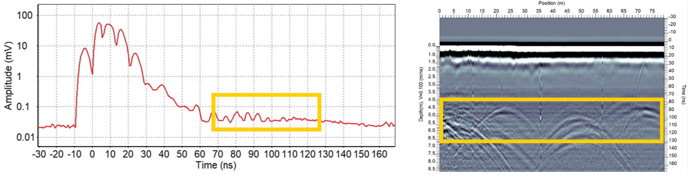
After the GPR signals have attenuated down to the background noise level, it is possible to see signals that reflected from objects above the surface such as trees, buildings, ceilings (when the GPR survey is conducted inside a building) and canopies. These reflections are called “air waves” because the signals travel through air at the speed of light. Air waves are commonly seen when the time window is much larger than the depth of penetration (Figure 3).
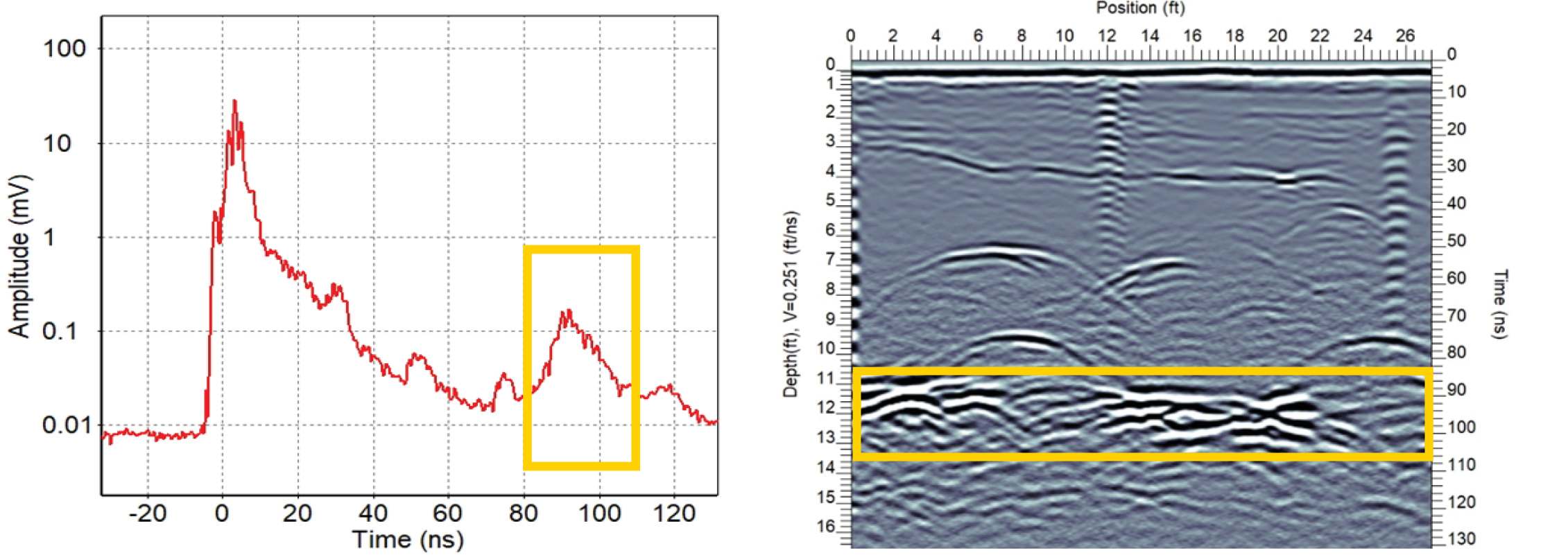
There are times when amplitude events at later times on an ATA plot turn out to be real subsurface reflectors (Figure 4). One of the great benefits of ATA plots comes from being able to assess the relative amplitude of signals that appear in the GPR cross- section. As part of interpretation, the likelihood that a deep weak signal is a true subsurface target can be weighed.
While we will not illustrate it here, displaying the ATA plot of a section before and after the application of time varying gain functions will help assess the reliability of the final cross-section when weak signals are strongly amplified.
Conclusion
ATA plots are available in the Processing module of the EKKO_Project™ software. This type of processing provides a powerful tool enabling users to make the best possible interpretation of the GPR data. The ability to differentiate noise from real subsurface reflectors, while not always easy to determine, means that the value of the GPR data is enhanced for the end use. The real value for everyone is to avoid mis-interpretation of data. To learn more about ATA plots and other powerful interpretation aids, contact us or see one of our on-line videos on data analysis.


